Fast Audio Video World Models: Part 2

Intro

This week at OWL we explored autoencoder enhancements and spent an uncomfortable amount of time trying to get KV caching working (almost there!) to speed up our Diffusion World Model. Today's blog post will cover our new technique for squeezing performance out of smaller DWMs and some things we found while looking into distillation to solve the KV caching problem.

TLDR

We trained an autoencoder with depth maps in the latent. It resulted in far better depth consistency in downstream generations. Next we're training with optical flow as well, and solving the KV cache problem.

DWMs and Latency

The "lag" of a Diffusion World Model scales with O(NTD), where N = number of tokens per frame, T = timesteps for diffusion and D = model depth. In this blog we are going to talk about how we are planning on improving all of these, as well as an aside on some new VAE stuff we did. At this rate it may seem like all of our blog posts are about Autoencoders, but we're fairly certain that after we fix high frequency generative loss, this issue should mostly resolve itself.

Shrinking N

Our primary focus in our autoencoder work has been on pushing sample size as small as possible while preserving sample quality to the best of our ability. Every additional push on compression shrinks tokens by a factor of 4x. As a general observation, diffusion transformers work best when patch size is simply 1, so we will refer to pixel count as token count. Traditional popular autoencoders (i.e. Flux, Stable Diffusion) only compress images by a factor of 8x, meaning a token reduction of 64x. We have two branches we are currently exploring:

• A 64x autoencoder that reduces frames to 8x8, ala 4096x token reduction (64 tokens)
• A 128x autoencoder to 4x4, ala 16384x token reduction (16 tokens)

In both cases we push channel count to 128, which the literature suggests can slow down training significantly, even though it leads to better downstream performance. Diffusion training is already brutally slow, but in our search for smaller token counts, this might honestly be fine. We’ve personally found that with 8x8 latents, this is true, but for some reason when you’re using 4x4 latents you get faster early training but worse final performance. In all honesty, with the speeds we get, we are considering just settling for 8x8, but we have some further experiments to run before we come to a final conclusion on this. This single change can be a near 4x multiplier in FPS, as it means diffusing 16 tokens vs. 64 tokens. 

You may wonder why we only do spatial compression and not temporal compression. The reason here is simply that KV caching and frame-by-frame generation becomes impossible with a traditional temporal autoencoder. We are actively exploring latent translation mechanisms between our autoencoder and Wan 2.1B, and we plan to release a blog post on this along with more exotic forms of model distillation in a few weeks. Temporal compression can reduce token-count even further, if you can find a way to integrate new frames into it without breaking caching.

As an aside, it’s worth bearing in mind that there is somewhat of a paradigm shift when going from many tokens, few channels to few tokens, many channels. As such, some methods that work for the former might not work for the latter. The biggest slowdown in our research thus far has been discovering these kinds of inconsistencies and pivoting quickly when we encounter them. There is still further research to be done here ahead of our first major model release, and we are actively looking for contributors and full-time researchers who are interested in pushing image compression to its limits. 

Shrinking T

Diffusion distillation is a pretty popular thing. Unlike traditional distillation where you distill a big model into a small model, in diffusion distillation you distill a many step model into a few step model. We have explored two main methods. The one we previously had the most experience with was shortcut diffusion. This seemed to work relatively well on images, and had the added benefit of being something you could tie into pretraining, rather than being posttraining. While we found this to be nice for our diffusion decoder, it was not particularly helpful for our world models. To this end, we have settled on Distribution Matching Distillation, as it has a good track record in the video diffusion literature and is quite sample efficient and simple to implement as far as post training techniques go. The paper also claims to enable one step generation. We will start with a quick rundown of how DMD works.

DMD

Take your model. Copy your model. Copy it again. One of these is your “real score function”, one is your “fake score function”, and one is your student. TL;DR of this is that your real score function predicts your ground truth videos given noisy videos. Oh wait, the teacher already does that! We can leave it as is. The fake score function predicts “fake” videos given noisy videos. The teacher already knows how to go from noise to real videos. The score function is going to need to learn how to go from noise to fake videos. 

What are “fakes” you ask? Well they’re generations made by the student. This is sort of like a GAN with extra steps. The student generates some “fake” videos, the fake score function learns how to go from noise to those fakes. There’s unbalanced training here where you train the fake score function many (we do 5) times for every time you train the student/generator. This is literally just standard rectified flow training, but looking at “fake” generations instead of ground truth videos. Let’s call this the critic. Then it’s the student’s turn.

We get the score from the teacher, and the score from the critic. One tells you how to “go to” real samples, the other tells you how to “go to” student samples. Get the difference. This directly serves as your gradient. Backprop through both the teacher and the critic, and it lets you align the “noise to fake” flow with the “noise to real” flow directly. As a fun aside this is how you use a direct gradient in PyTorch. When you differentiate, the terms all cancel out and you just get the gradient you want directly.

Back to Shrinking T

With DMD you can get high quality generations in 4 steps, and sometimes even ok-ish generations in 1 step. We’re probably going to go with 2 or 3 depending on the situation. For our base model, we generally found you needed at least 16 steps to get passable frames, so this is around a 10x speed increase. Pretty solid!

Shrinking D

In a transformer model, the depth of the model generally cannot be parallelized. You wait for every layer to finish before moving on to the next layer. If you can halve the layers, you double the speed. There are two main things to explore if one wants to reduce D. One is model distillation and more efficient architectures, the other is feature extraction on the input data to “ease” the model into training with inductive biases. We have some preliminary findings on both of these that will guide our future research into this topic. 

Efficient Architectures

UNets are known to be faster than transformers, but with tiny latents it is unclear how we would exactly use convolutions. It seems to be common knowledge that convolutional models are better at smaller scales (likely due to inductive biases), but that transformer models dominate as you scale. UViTs try to buff transformers with the benefits of UNets by copying over the residual structure. Interestingly UViT seems to have the same problems as UNets, in that it doesn’t actually scale (at all). The UViT paper does not hide this fact. They find optimal performance at 13 layers. This effectively simplifies trading off depth for model width. This in turn simplifies trading off FPS for VRAM. We will be doing more sweeps in due time to fully explore scaling laws for the low token high channel regime with world models. More news on this in the future!

Inductive Biases

As previously mentioned, the most likely culprit for CNNs being better at small scales is their inductive biases in regards to working with images and videos. As such, it makes sense to think about the kinds of inductive biases we can give our DWM as-is. The simplest is to slightly modify its training objective. In the VideoJAM paper they found that small diffusion video models can hit far above their weight class if you train them to also generate the optical flow along with some existing videos. We tried this initially in the same way they did: doing channel concatenation on separately encoded optical flows. This did not work at all, likely because increasing the channel count to 256 entirely killed diffusability. Our next idea was to just start encoding things directly into the latent, such that channel count did not need to be increased.

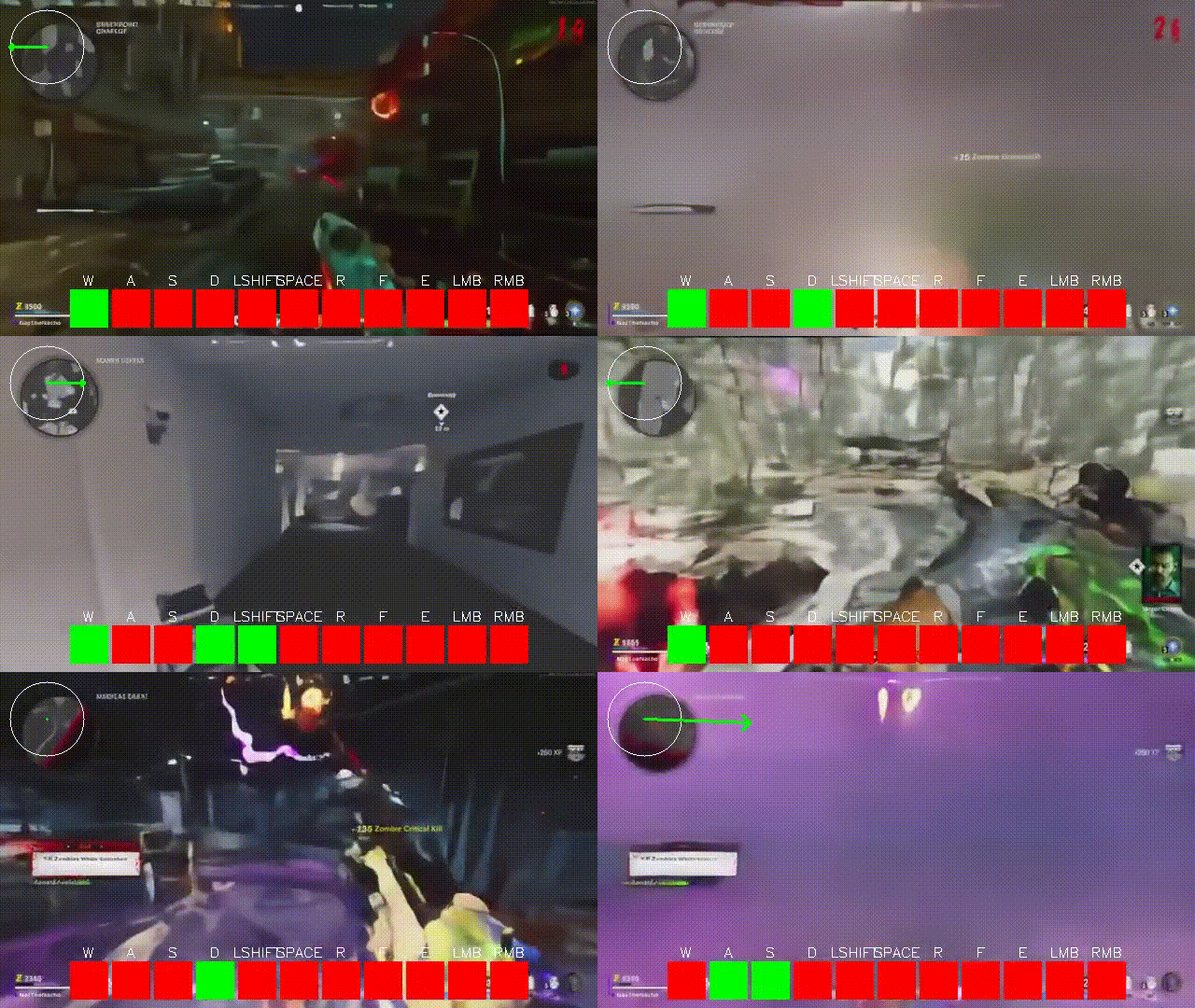
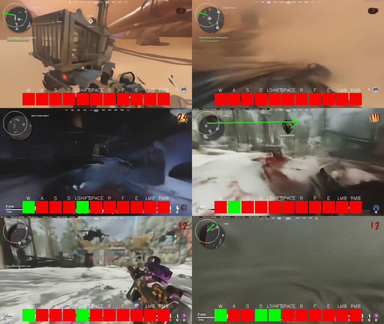
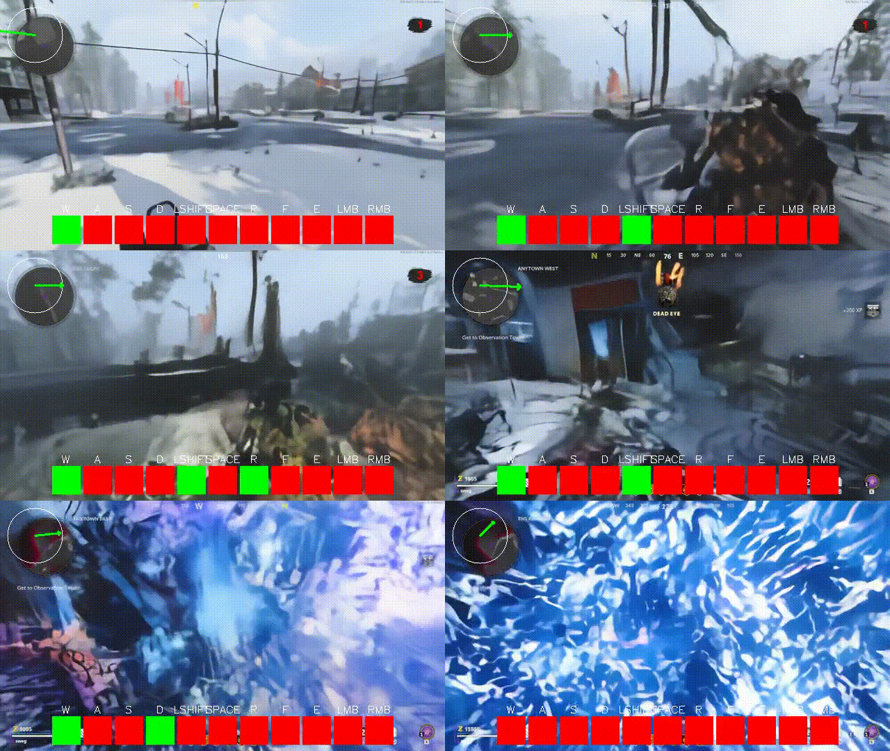
This led us to training an autoencoder that took image + depth maps rather than just images, compressing into a single 8x8 latent with 128 channels. We then trained a 1B diffusion transformer on these latents. Our results were… weird. The model learned to generate samples with consistent depth extremely early into training. For context, with our RGB only generations, we don’t expect to see *anything* until at least 30-50k steps into training. 

First, the norm:

Second, what we got with depth supervision:

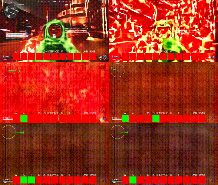
It’s pretty clear that depth supervision is helpful, however: we also got a lot of strange artifacts with depth supervision. Here’s two samples from way later in training. One that was quite good, and one that was quite bad. In all honesty, 90% of samples looked like the second one.

It seems like depth maps really do poorly when you’re inside or there's any particle effects going on. That being said, for the samples where it worked, it *really* worked. We think that having a better depth model and more data should alleviate these issues, and are actively working on this right now. Ahead of that we have trained an autoencoder on flow + depth + RGB and are going to be training a world model with it soon.

KV Caching: The Holy Grail

Everything I’ve listed above can get you to ~30fps. But there’s one more thing that, if solved, will get you past 400fps: KV caching. For us, there are two forms of KV caching for World Models: weak KV caching, and strong KV caching. Before getting into this, we should reiterate why you can’t KV cache in a traditional Diffusion World Model. Diffusion forcing requires history frames to be noised. The motivation behind this is that it prevents the model from focusing too much on high frequency information in the history. Once the history becomes primarily generated (long rollouts), the high frequency features in the latents reveal generation artifacts and errors. The model sees these, and it causes a distribution shift that results in a complete decoherence from accumulating error. The small errors compound into huge errors.

For the sake of clarity we will differentiate diffusion steps and frame steps. Diffusion steps are when we have some fixed history in a sliding window and are denoising the last frame. Frame steps are after we finish denoising and generating frames, and move onto subsequent frames, shifting our context window by one to the right. 

The immediate solution to the accumulating error problem as presented in the original diffusion forcing paper was to renoise previous frames. The worst part of this is that you have to *renoise* the history, and as such the previous frames must be reprocessed with new noise every frame step, drastically slowing down sampling speed. So what solutions do we have?

Weak KV Caching

An immediate observation is that, if you are using block-causal attention, you are only renoising the previous frames every frame step. They do not need to be reprocessed during the sampling steps of an individual frame. To this end we can cache on the first diffusion step, and as a result all subsequent diffusion steps are practically instant as the time complexity effectively goes from O(nmt) to O(nm) + O(t), where m is the number of frames and n is the number of tokens per frame. This speeds up inference when we are doing many diffusion steps but isn’t particularly interesting after one implements DMD and reduces diffusion steps regardless, as at that point O(t) is just O(1) anyways. So with weak KV caching + diffusion distillation we are down to O(nm). What next?

Conclusion

If you'd like to help with any of these projects or join in on the lively discussions that actively take place on our server, please join here! While you can join as a volunteer whenever you'd like, we are also taking applications for full-time positions here. If you are interested in the future of entertainment experiences and want to join one of the fastest moving teams in the space, please do apply!